TTS Evaluation: Preference Test

Evaluating TTS systems can be tricky. There are two types of subjective tests commonly used in TTS papers: absolute ratings, such as naturalness Mean Opinion Score (MOS), and preference tests. In absolute ratings, a single sample is presented to a listener who is asked to rate it on a 5-point Likert scale. While such scores are useful to get a sense of the overall quality of a TTS system (e.g. how good is it compared to natural speech?), they are not always suitable to assess finer quality differences. In such cases, we use preference tests. In this post, we describe the process of setting up and reporting TTS preference tests in our lab.

What is a preference test?

We use preference tests to compare two TTS systems: A, and B. For example, consider a TTS system trained on Modern Standard Arabic data. In system A, we omit all diacritics. In system B, we use ground-truth diacritics. Which system produces better speech?
After training the two systems, we randomly sample 15 to 20 texts from the test set, and generate speech by the two systems.

Setting up the test

We use Gradio for setting up the test. Listeners are presented with a pair of audios, generated by systems A and B using the same text. The order of samples is randomized for each listener, as well as the order of the systems for each sample, to avoid any potential bias from listening order.
We also insert two control samples, where we present a clearly better audio (e.g. ground truth) and a low-quality audio (does not have to be generated by either A or B; it has to be clearly worse than the other one). These allow us to assess whether listeners are paying attention and actually listening to the audios. This is especially important in paid crowd-sourcing platforms where there is incentive to complete tasks quickly without engaging with them.
We share the scripts to replicate our Gradio setup in this GitHub repo. We then compute and plot the mean proportions of votes for A, B, and No Preference across all 20 samples, with confidence intervals (CIs) for each, using the t-distribution (because the sample size is small). Below are all the steps, with an example.

Aggregating the ratings

Suppose we have n=20 samples, each rated by r=10 raters. The raters choose an option from A, B, No Preference (NP). For each sample $i \in [1-20]$, we calculate the proportion who selected each category. For example, suppose we have the following ratings for sample 1: $$ [A, A, NP, A, B, A, A, B, NP, A] $$ The proportion of raters who selected A, B, and NP for sample 1, is $p_1^A=6/10=0.6$, $p_1^B=0.2$, and $p_1^{NP}=0.2$, respectively. This means that for sample 1, more than half the listeners prefer system A.
Once we calculate the proportions for all 20 samples, we will have 20 proportions for each category. We can now utilize the Central Limit Theorem to estimate confidence intervals:

Central Limit Theorem: The distribution of sample means approaches the normal distribution as the sample size increases, regardless of the population distribution.

What this means is that that sample means (i.e., a sample of 10 ratings) will be approximately normally distributed, with mean equal to the true population mean (i.e., the mean of all possible ratings). We can therefore calculate the means of the ratings for each category and calculate confidence intervals using the normal distribution. However, since our sample size is relatively small, Student's t-distribution provides a better estimate of the confidence interval. To proceed, we calculate the mean proportion for each category; for example, for category A, we have the 20 proportions calculated by averaging the 10 ratings for each sample: $\{ p_1^A, p_2^A, ... , p_{20}^A\}$. We calculate the mean proportion (with n=20): $$ \bar{p}^A = \frac{1}{n} \sum_{i=1}^{n} p_i^A $$ We then calculate the standarad deviation $$ s_A = \sqrt{ \frac{1}{n - 1} \sum_{i=1}^{n} \left( p_i^A - \bar{p}^A \right)^2 } , $$ and the standard error $$ SE_A = \frac{s_A}{\sqrt{n}} $$ To compute the two-tailed 95% cofidence interval using the t-distribution, we first obtain the t-value. We can use an online tool like this one to get the t-value for p=0.05 (corresponds to 95% confidence interval) and degrees of freedom = $n-1 =19$. This turns out to be $t=2.093$. The confidence interval can be obtained by multiplying the t-value by the standard error: $$ \bar{p}^A \pm 2.093 \cdot SE_A $$ We repeat the calculations for $\bar{p}^B$ and $\bar{p}^{NP}$.

Plotting the results

Once the mean proportions and confidence intervals are obrained, we can plot a bar chart with error bars corresponding to the confidence intervals. In the example below, the confidence intervals for A and B are overlapping, suggesting that the difference between them may not be statistically significant.

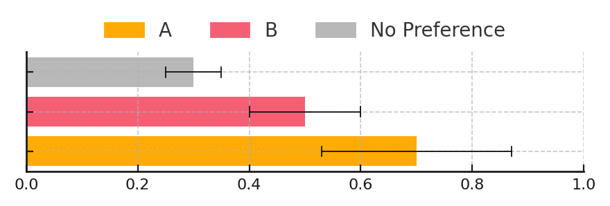
import matplotlib.pyplot as plt

categories = ['A', 'B', 'No Preference']
means = [0.7, 0.5, 0.3]
errors = [0.17, 0.1, 0.05] 
colors = ['#FFAB05', '#f55f74', '#b8b8b8']

plt.figure(figsize=(4.5, 1.8))

for i, (mean, error, color) in enumerate(zip(means, errors, colors)):
    plt.barh(i, mean, color=color, height=0.75)
    plt.errorbar(mean, i, xerr=error, fmt='none', ecolor='black', elinewidth=0.6, capsize=0)

    # Add vertical ticks at each end of the error bars
    tick_height = 0.25
    plt.plot([mean - error, mean - error], [i - tick_height / 2, i + tick_height / 2], color='black', linewidth=0.6)
    plt.plot([mean + error, mean + error], [i - tick_height / 2, i + tick_height / 2], color='black', linewidth=0.6)

#legend
handles = [plt.Rectangle((0, 0), 1, 1, color=color) for color in colors]
plt.legend(handles, categories, loc='upper center', bbox_to_anchor=(0.5, 1.4), ncol=3, frameon=False)

# axis settings
plt.xticks(fontsize=8)
plt.gca().set_yticks(range(len(categories)))
plt.gca().set_yticklabels([]) 
plt.xlim(0, 1)
plt.grid(axis='x', linestyle='--', alpha=0.7)

# display figure
plt.tight_layout()
plt.show()